
GDC talk: Scalable Real-Time Ray Traced Global Illumination for Large Scenes
.jpg) |
At the end of March on GDC we presented our solution for Global Illumination. The presentation is available on GDC vault, but we want to detail it to you in written form.
One of the most important aspects of game development, besides introducing new content is innovating new features and ensuring they run fast and efficiently. Today, we would like to talk to you about Scalable, Real-Time, Global Illumination for Large Scenes, and how this affects the dynamic environments inside Enlisted.
1. OVERVIEW
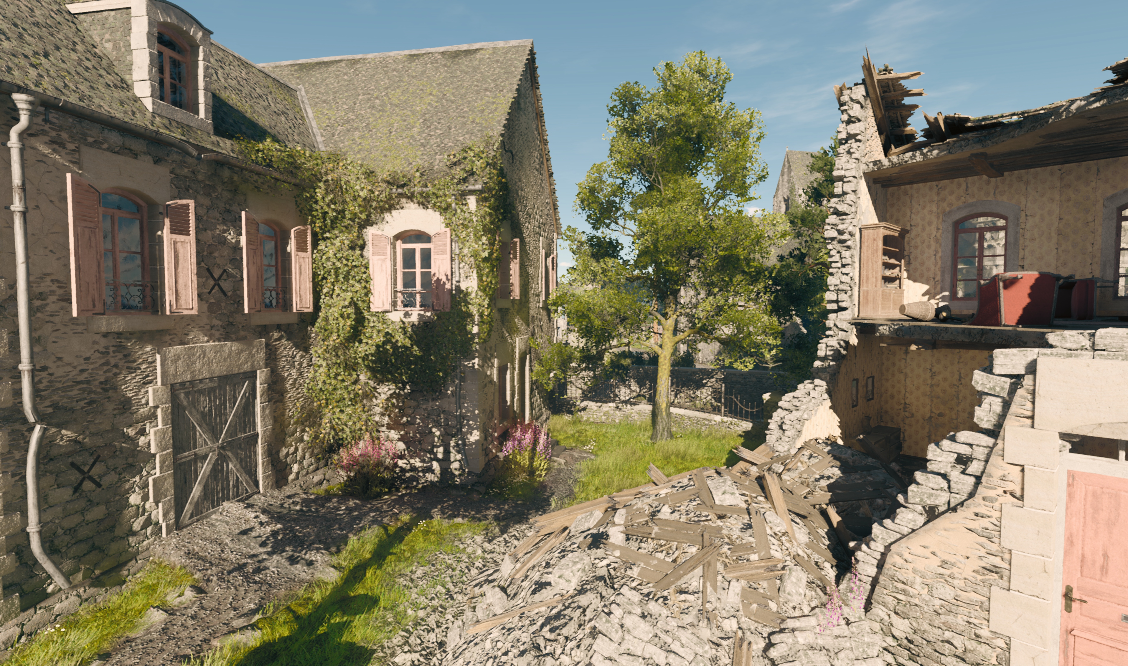
Rich and dynamic environments make up all fundamental aspects of Enlisted. There are a huge number of variations in seasonal and weather conditions, regional climate, time of day, amongst other items, that all must come together seamlessly over a single-large scale map area (up to 64 sq.km) with destructible environments, terrain features, constructable and static fortifications, and a multitude of other entities. The most challenging aspect of this is not only making sure that lighting is realistic, immersive, natural in appearance, but also that it suits the time of day and climate of the Native battle scene being depicted - both indoors and out. Enlisted was designed to feature all of these core elements within its environments, so it was important that we found a solution that worked well without a major compromise to performance for players.
Solution:
Our solution introduces a new dynamic for real-time Illumination combining the quality of a precomputed indirect lighting with one similar performance to a modern screen-space techniques while at the same time capable of supporting very large scenes for static (or semi-dynamic, i.e. which changes slowly) lights with very moderate memory requirements to the player.
This was accomplished by utilizing a Voxelized lit scene around the camera which allows for multiple bounces from indirect light and from numerous light sources (including Sky Light) in less than one millisecond on current generation consoles (and 0.57msec time on modern PC GPUs (GTX 1070)) - with the ability to scale to RTX cores in order to increase quality.
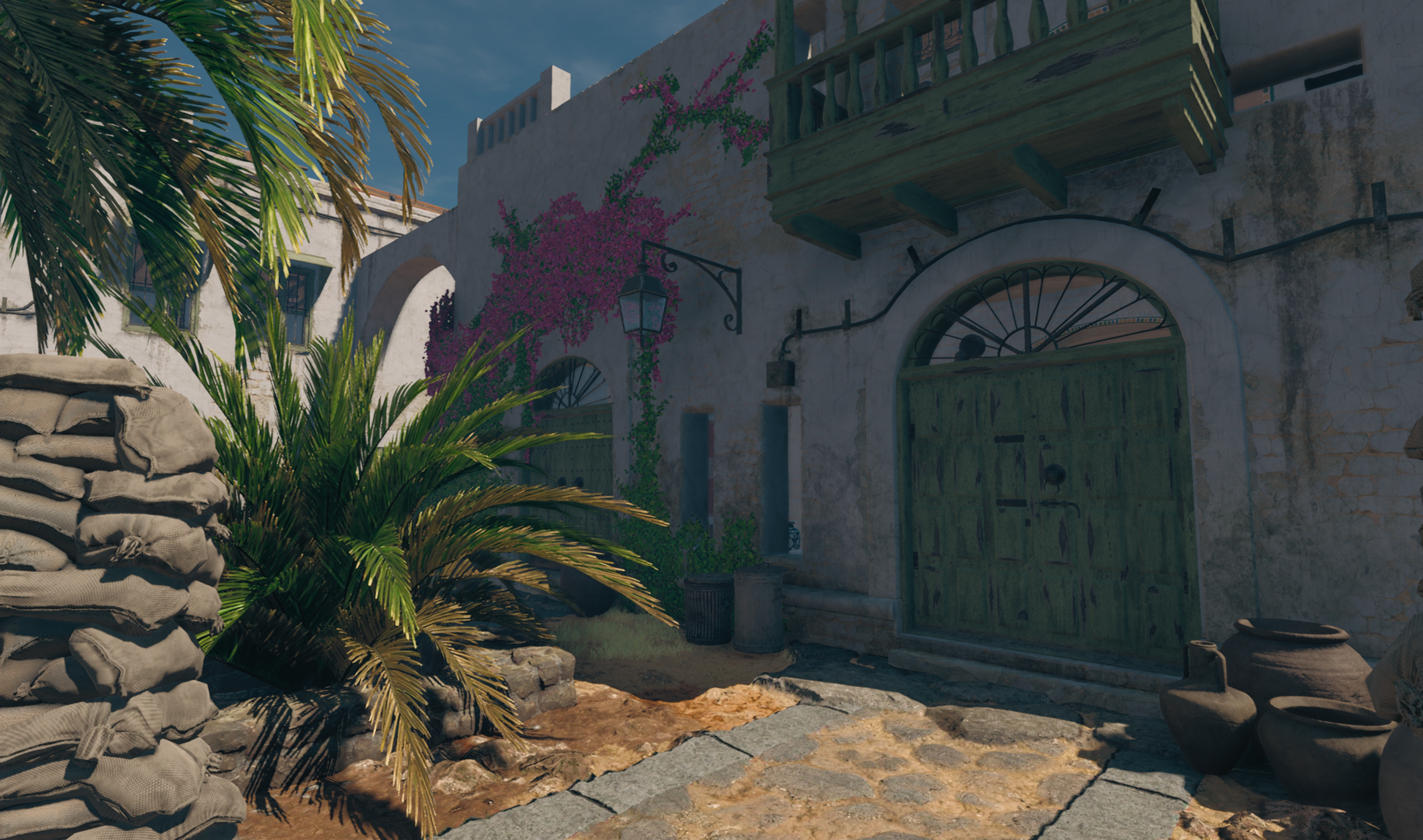
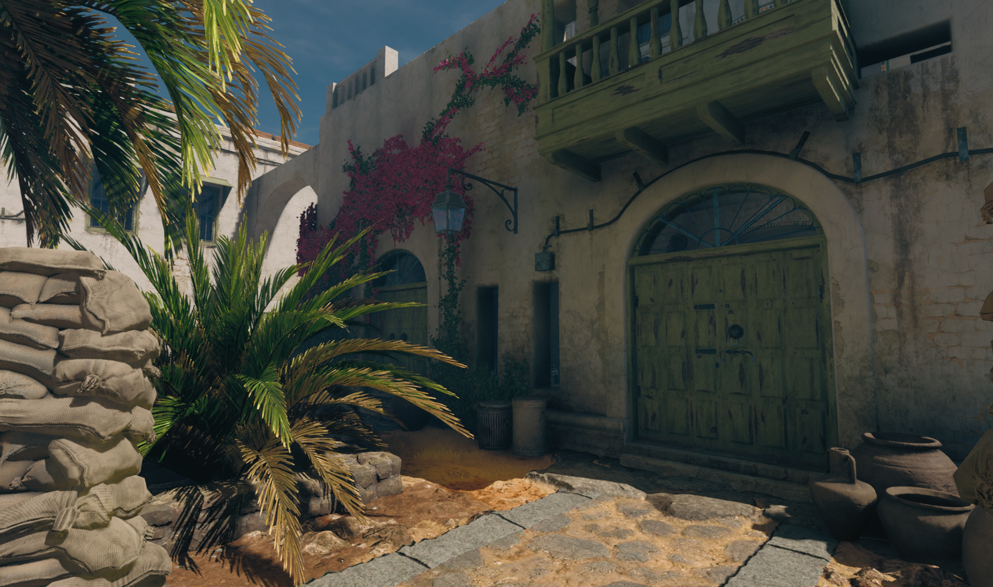
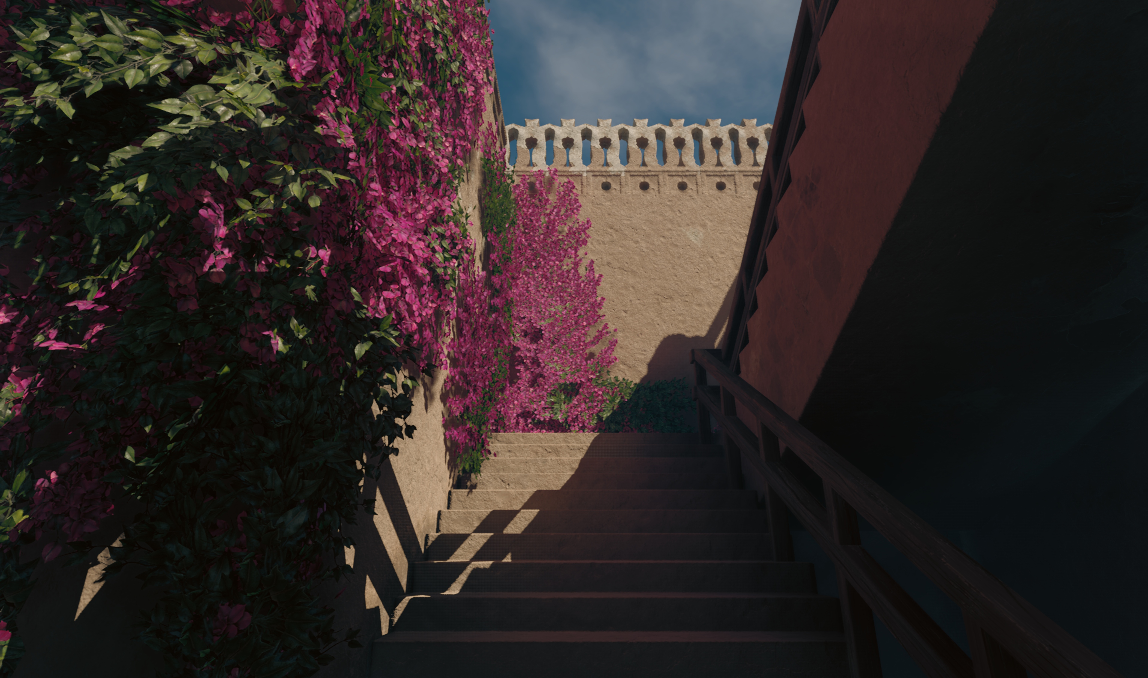
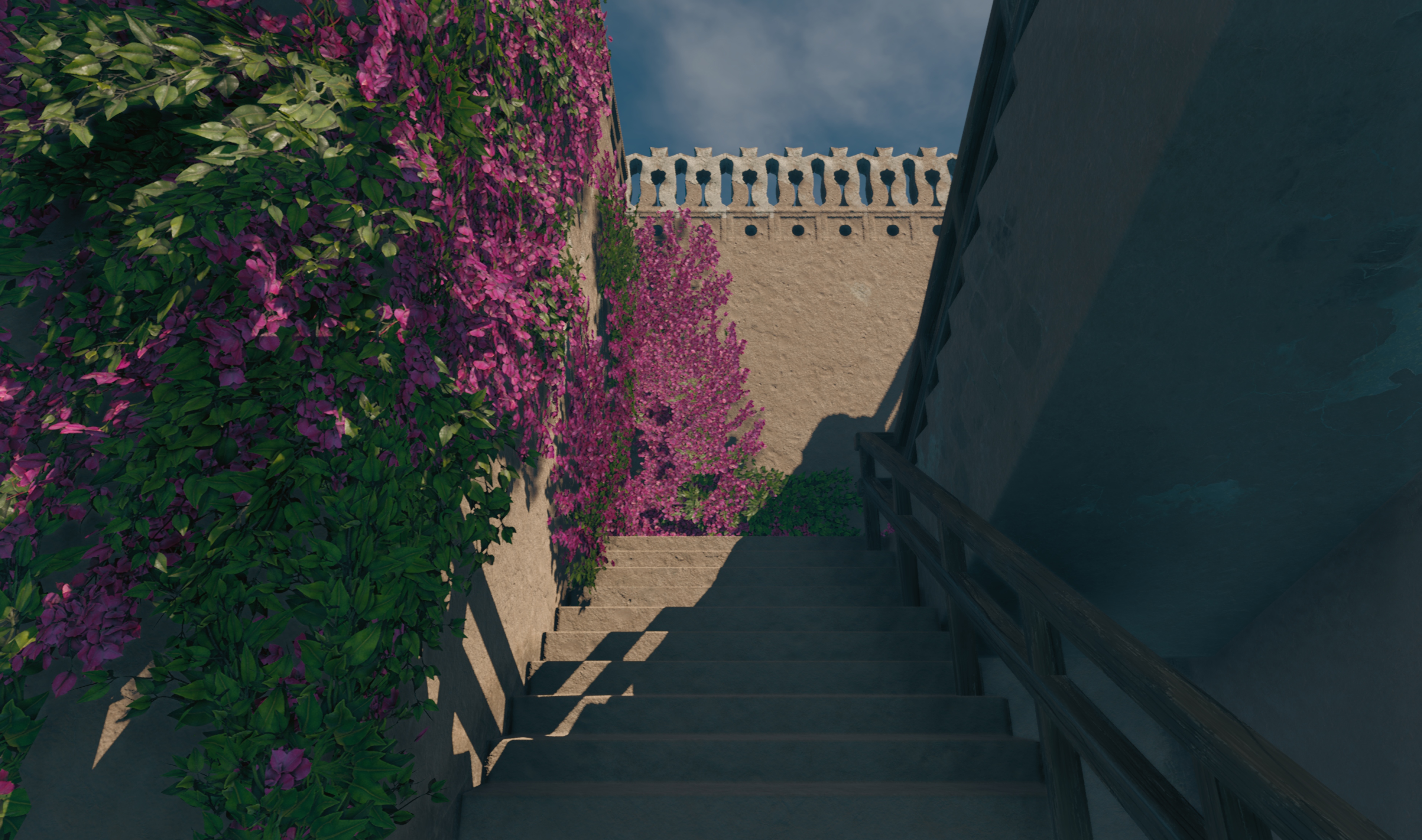
| ON | OFF |
|
|
|
| ON | OFF |
|
|
|
| ON | OFF |
By introducing these new algorithms and data structures to compute global illumination from semi-dynamic environments (potentially infinite scale in real-time). We relied on a screen-space G-buffer to temporally fill several nested 3d-grids (cascades) representing the scene around the player, and several nested 3d grids of light information around the player as well. In its simplest implementation this algorithm requires zero knowledge about any particular scene, (just as most of screen-space techniques) but at the same time it produces out-of-screen details and doesn’t suffer from aliasing artifacts.
It also doesn’t require any pre-computation or knowledge about the content of the scenes, but additional information (such as light probes, or proxy geometry, or minimal height map/floor) which usually exist in games enhances the speed of temporal convergence and quality. We then applied ray tracing techniques to this data structure to efficiently sample radiance on world space rays, with correct visibility information, directly within compute shaders to compute 3d grid of indirect lighting + sky light in form of ambient cubes or spherical harmonics. From this basis we then use well-known GPU algorithms to efficiently gather real-time viewer-dependent diffuse illumination onto both static and dynamic objects.
 |
 |
 |
|
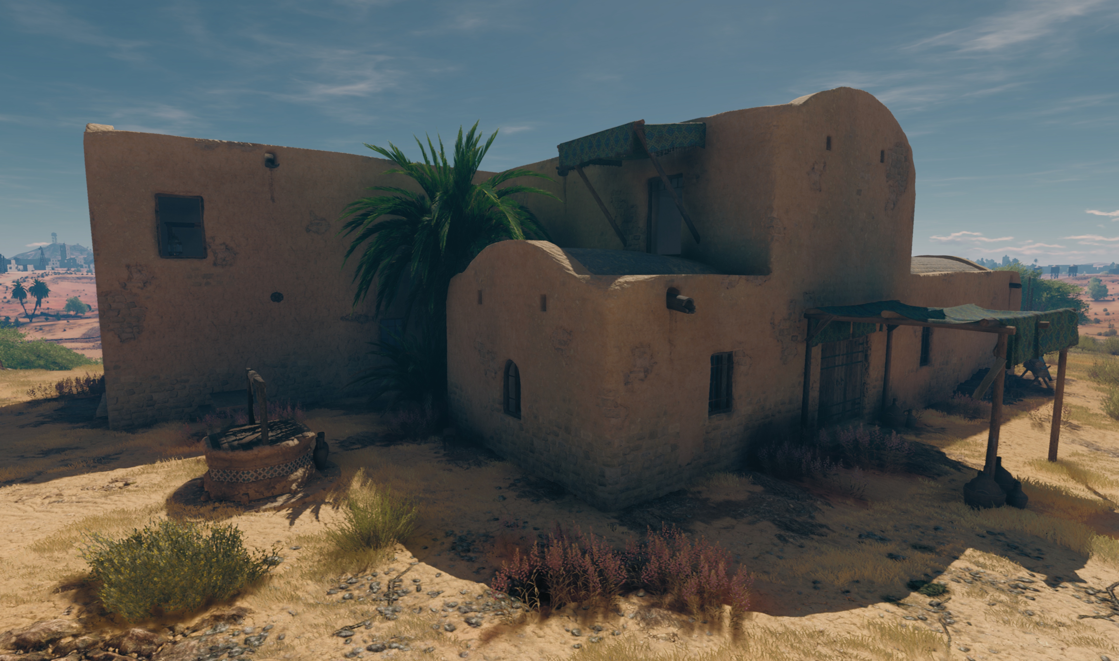
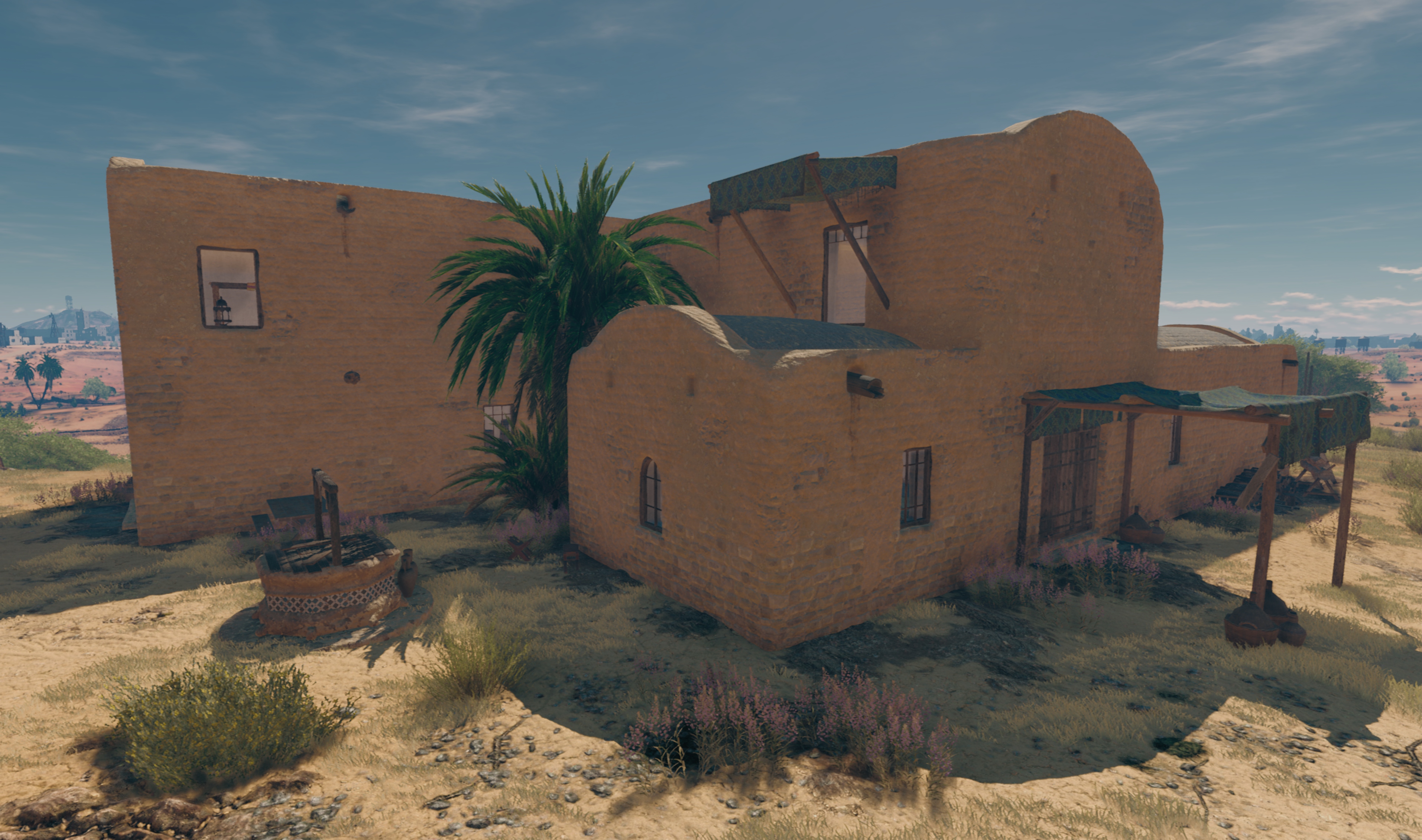
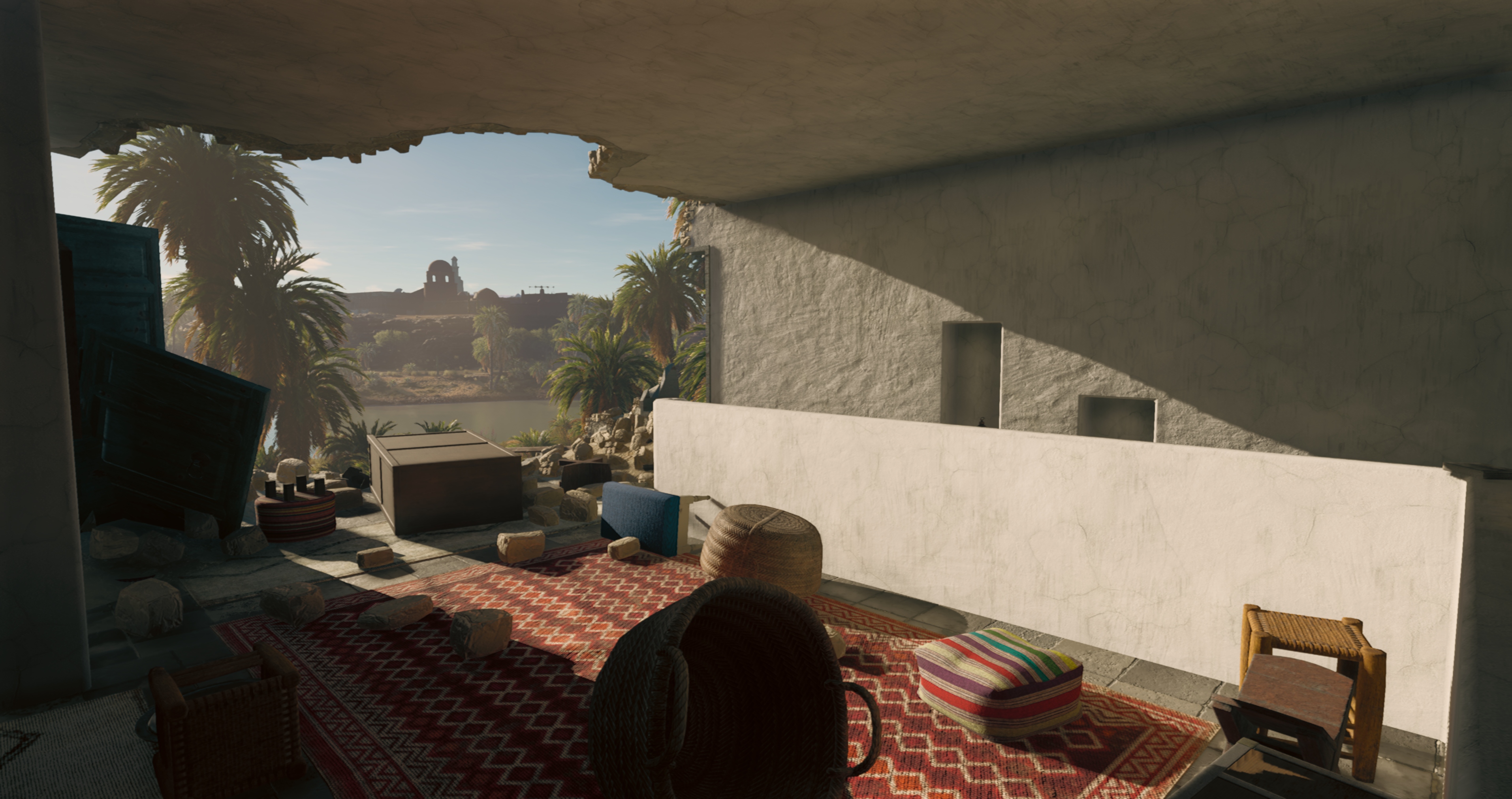
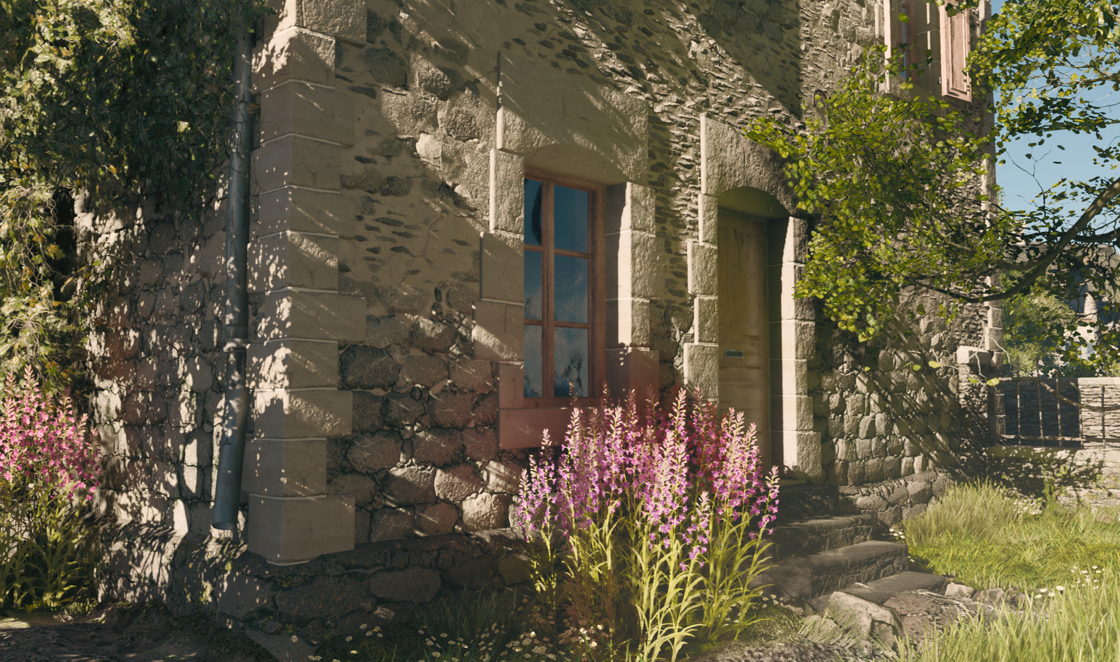
| From left to right: "Tunisia", location size over 16sq km; Enlisted sample image, close-upscene, Normandy; Same location outside building; |
|||
TECHNICAL ELEMENTS
2. ALGORITHM OVERVIEW
A scene’s continuous irradiance volume map encodes incoming indirect (bounce) and skylight irradiance for all chosen directions in the scene.
We build a discrete representation of this distribution, and so we require a discretization of positions in space and directions. For directions, typical representations are Spherical Harmonics or Ambient Cube [McTaggart 2004]. While spherical harmonics are well defined and allows extendable resolutions, for our purposes we have chosen ambient cubes. Ambient Cubes allows us to exploit hardware trilinear filtering, and compression of representation, however the chosen representation consists of just 6 directions. We discretize irradiance map in space using a regular grid of light voxels inside the box around the camera. This regular structure (in combination with ambient cubes) allows us to exploit hardware trilinear filtering. To enhance quality around the camera our irradiance map consists of several nested structures (3D clipmap, Figure 1). We then calculate incoming radiance in each visible cell in our discretized irradiance map. To do that, we ray cast thousands of rays in a scene, and so calculate incoming radiance in each direction using Monte Carlo integration. To speed up ray casting, and to get incoming radiance for each ray we use discretized scene around the camera, as a set of nested grids of voxels (3d-clipmap, see Figure 4) around the camera, similar to [Panteleev 2014]. We store only already lit voxels in our scene representation, without any directional opacity information. Our main innovation is that we update this 3d-clipmap scene representation directly from G-buffer, stochastically choosing some pixels on screen in each frame, effectively performing temporal supersampling on each scene voxel. Since these pixels are relighting using already computed irradiance map (as well as direct lighting information) we effectively get multiple bounce information in our irradiance map (see Figure 8), with a potentially infinite number of bounces. Because our ray casting is bruteforce ray traversal in a voxel scene, we do not "skip" thin or complex geometry, like naive voxel cone tracing [Crassin et al. 2011], [Panteleev 2014] (see Figure 3), which also allows us to add sky light to our irradiance map. If a ray has missed, we use environment (specular) probes to get incoming radiance, or one sky environment probe, if probes are not available.
3. IRRADIANCE MAP OVERVIEW
3.1 Updating irradiance map implementation details
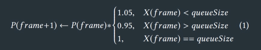
This 3d-clipmap (Figure 1) is addressed in a toroidal way (WRAP addressing in the case of hardware filtering) and when the camera moves, there is no need to copy or discard unchanged cells in a grid(s), just a "filling in" of new cells, see (Figure 2). We keep the center of our irradiance map in camera, but those centers do not have to be exactly aligned or exactly match each other. To simplify lighting with irradiance map we keep each finer level completely inside it’s coarser neighbor. For easier irradiance map memory management, we keep all levels of our clipmap of the same size in two dimensions (in our case in horizontal dimensions), which allows us to store the whole irradiance map in one volume atlas texture. Each frame we relight some visible cells of our irradiance map. We use a stochastic selection of visible cells, with probability based on it’s temporal age (time how long we have not updated the specific cell). The probability for each cell is chosen based on age ∗ random > P, where random is pseudo-random function returning numbers in [0..1], and is chosen based on the previous frame cells passed count X:
_alfa.png) |
Fig. 1. 3d clipmap around camera. From left to right: Box around the camera, lod0 (finest) size is 1/8 of the box size, lod1 is 1/4, lod2 size is the whole box. All textures are of the same size in texels but different sizes in the world space, so texel (voxel) size doubles each next level.
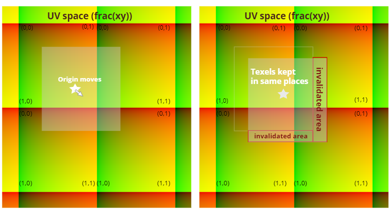 |
Fig. 2. When the clipmap texture origin moves we don’t copy or re-write any valid data.
 |
For visibility we use both frustum culling and occlusion based on hierarchical z-buffer [Hill11] We keep several limited queues for each criteria.
-
QueueA. Cells that have intersected with the scene. If a cell is visible and intersects (partially occluded) with an opaque scene, it usually affects the final picture more than a cell that is fully unoccluded (visible), and only intersecting cells are participating in light transfer.
-
QueueA′ . Cells that intersect scenes and have zero temporal age (never updated). It is important to keep something reasonable in any cell, since our updating algorithm is temporal, and a cell can change it’s visibility too quickly due to camera movement. Alternatively we could update the probability function f based on the current frame, not the previous one, but doing so would require more computational time than just filling both queues.
-
QueueB. Cells that do not intersect a scene. These cells can still affect the image, as dynamic and transparent geometry can be lit with them.
We then update irradiance map cells in all queues. ForQueueAandQueueA′ queues, we keep the total cells to process limited to the capacity of each queue, so we first update QueueA′ and then first N cells in QueueA, where N is capacity(QueueA) − occupied(QueueA′ ). We use compute shader to fill these queues, and then another compute shader (with dispatch indirect) to relight the queued cells. The size of queues defines the speed of convergence and the total performance cost of the algorithm. We ended up using 512-1024 cells for QueueA and 64-128 cells for QueueB.
3.2 Fill-in new cells in irradiance map implementation details
Each time we have to ’fill-in’ new cells in a irradiance map due to movement of the camera, we use the following algorithm. For each of the finer grid levels we initialize cells from a coarser level (since grids are nested). For the coarsest level, we initialize with ’new’ state.
We just raycast with small number of rays to get initial data.
3.3 Ray casting implementation details
We use compute shader to relit queued cells. Each compute shader runs parallel raycasting of different rays in different threads for each cell. For simplicity we use one thread group for each cell, and one thread for each ray, and then parallel reduction algorithm to accumulate results. We temporally accumulate results in the cell, with exponential weight based on the cell’s update age. It is technically possible to use voxel cone tracing to speed up lighting phase. However, we want to have accurate indirect and skylight in our irradiance map. Voxel cone tracing can report invalid ’partially occluded’ result in case of thin or complex obstacles (Figure 3).
_alfa.png) |
|
Fig. 3. a) cone tracing wrongly reports thin obstacle as ’partially occluded’, as it is thinner than cone size in a step. b) cone tracing wrongly reports two obstacles as ’partially occluded’, although the whole cone should not pass obstacles. |
4. SCENE REPRESENTATION IMPLEMENTATION DETAILS
Scene 3d-clipmap (Figure 4) is also addressed in a toroidal way (WRAP addressing in case of hardware filtering, Figure 2), and when the camera moves there is no need to copy or discard unchanged cells in a grid(s), just "fill in" any new cells. Initialize 3d clipmap (nested grid) as a set of volume textures. For simplification, we keep all levels of our clipmap of the same size in two horizontal dimensions, which allows us to store it in one volume atlas texture.
 |
 |
 |
 |
|
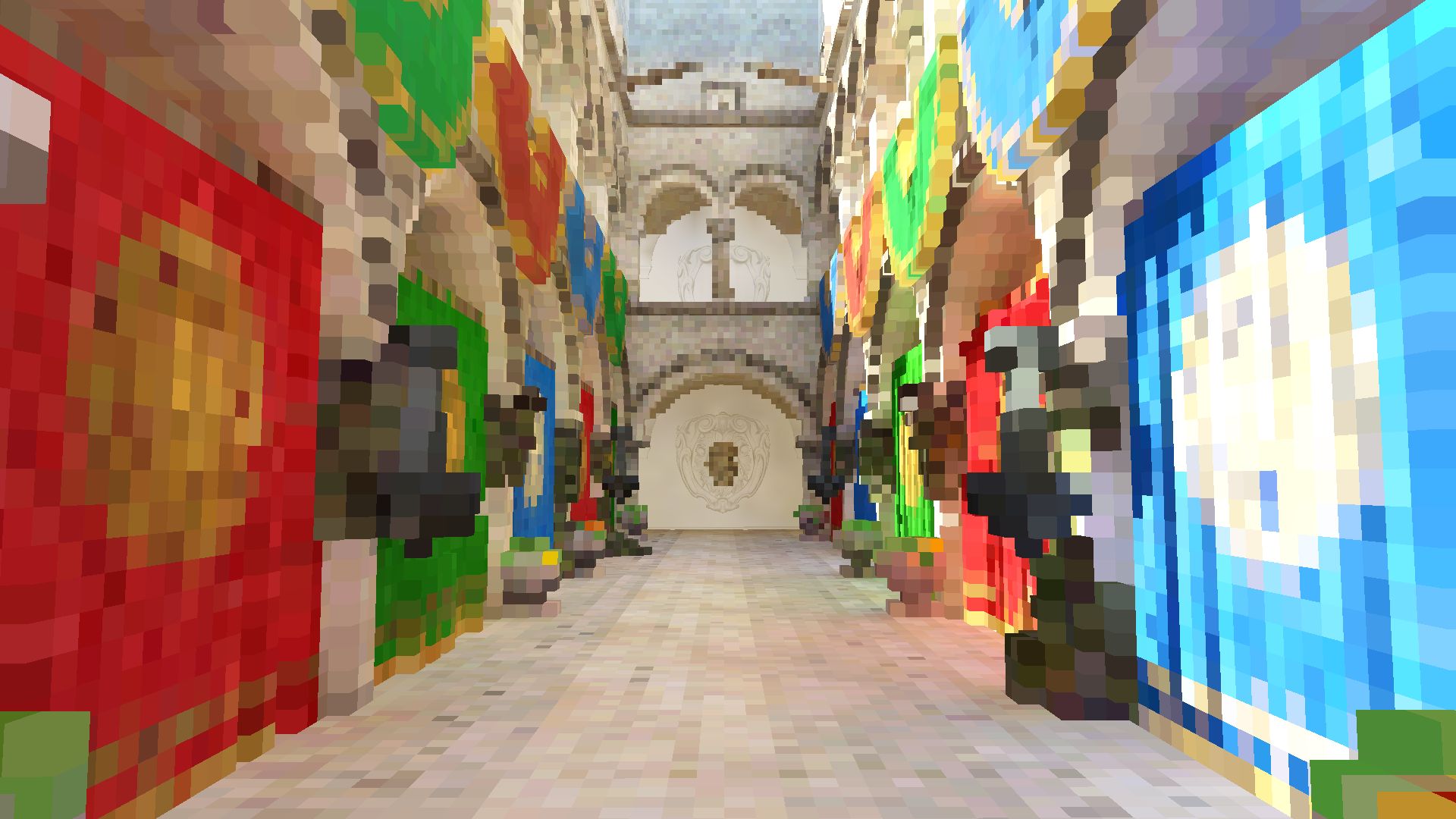
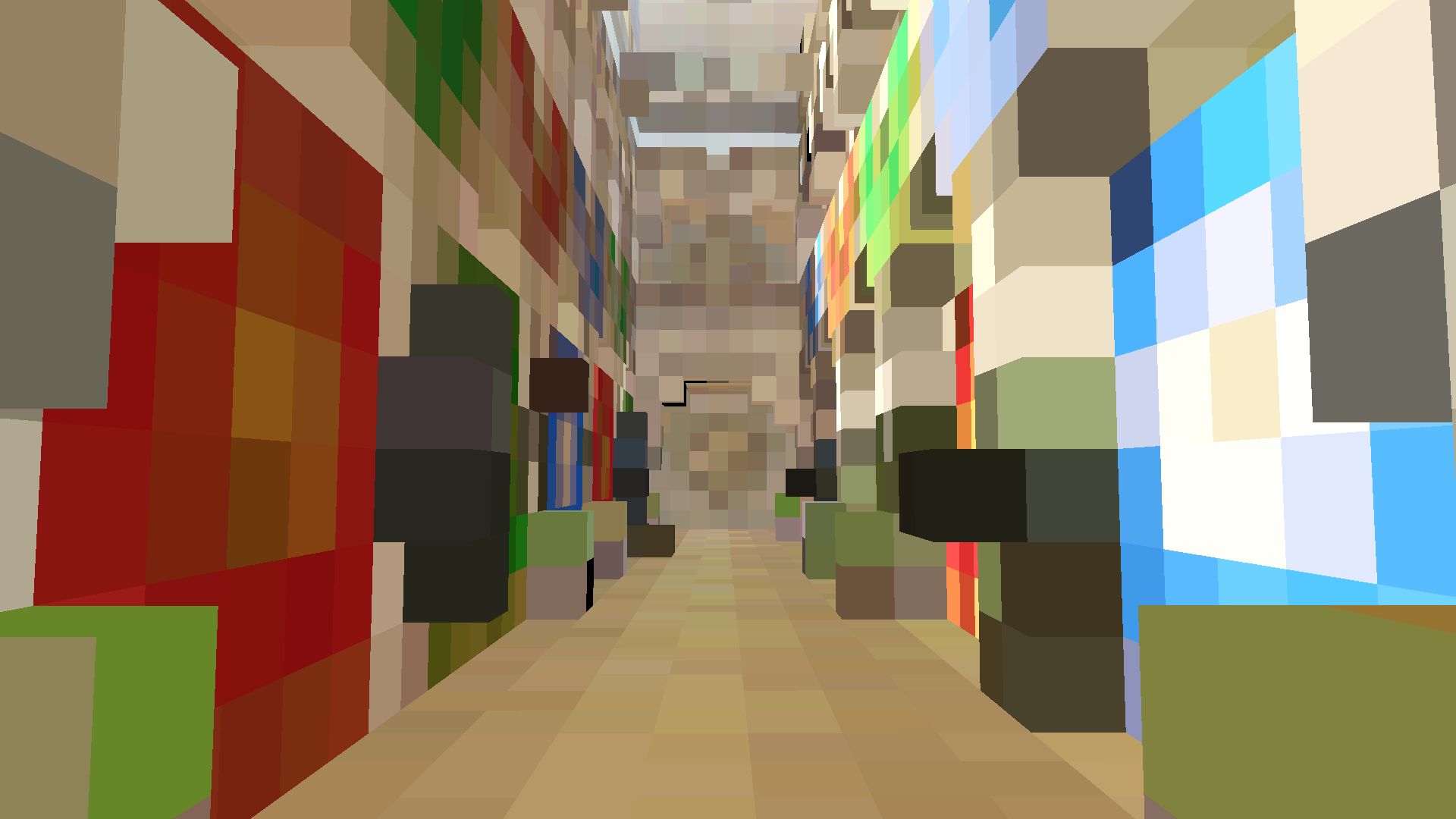
Fig. 4. Scene voxel representation clipmap, Sponza scene. Each grid has same texture dimensions and is nested inside coarser one in world space. Top-left: finest, bottom-right coarsest levels. |
|||
 |
 |
 |
|
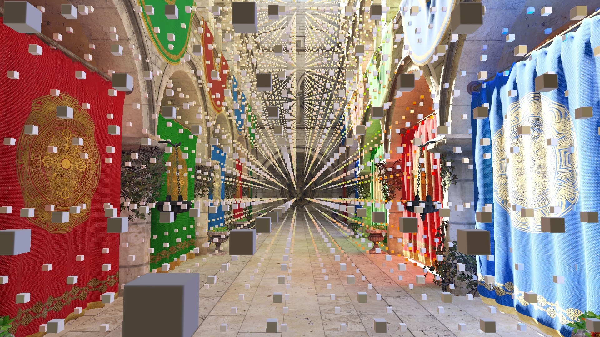
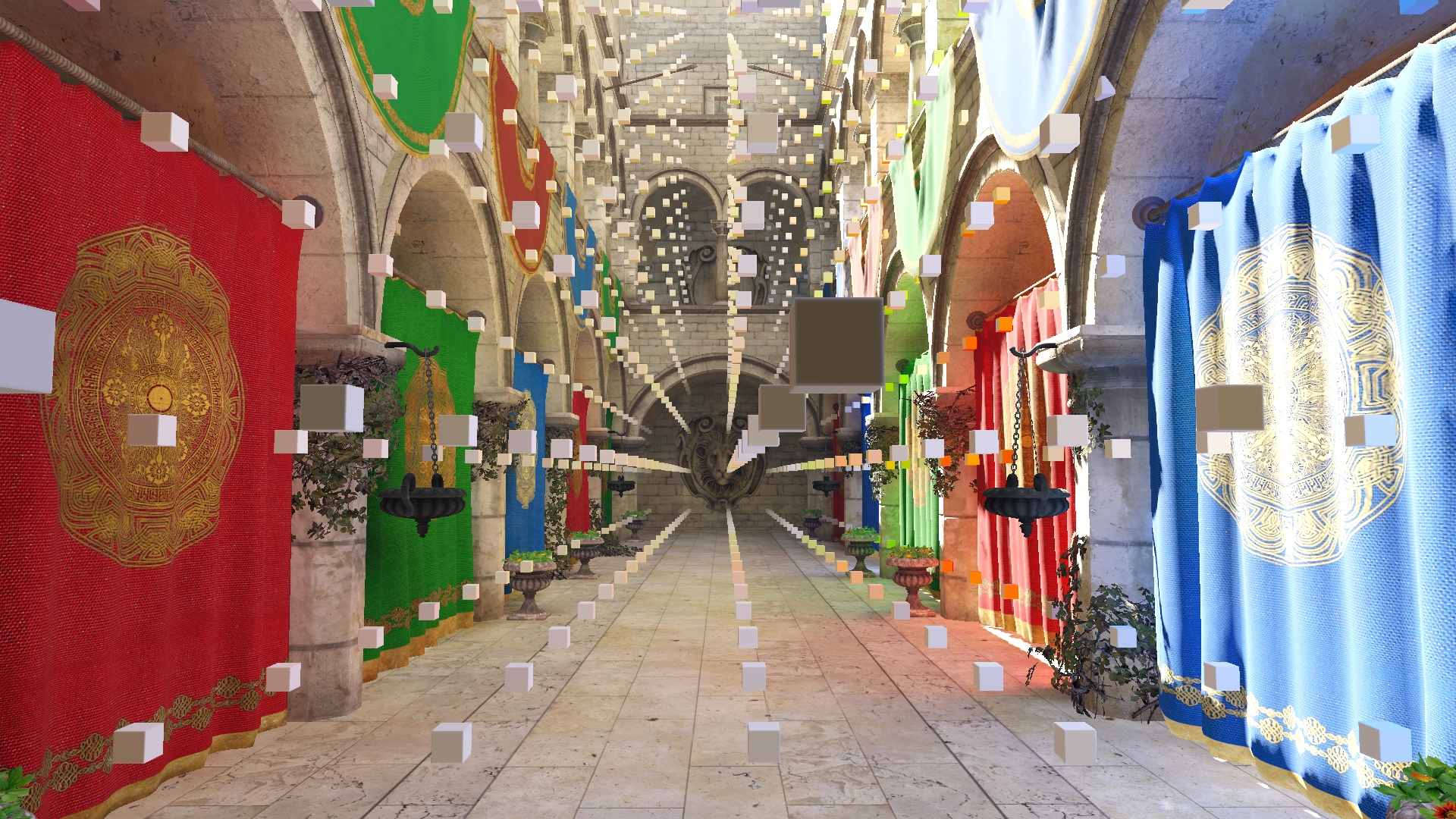
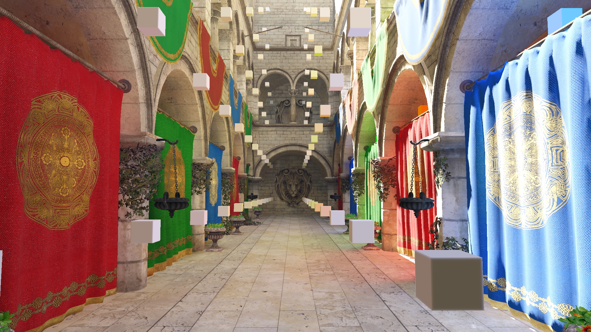
Fig. 5. Irradiance map clipmap. Small boxes are representing center of irradiance map texels and shaded with with value of each texel, and size is proportional to texel size. Top-left: the finest level. Bottom: the coarsest level. |
||
We also need to keep ’color’ and (optional) ’opacity’ information, for each we can use either alpha channel for texture formats with each that has that information or keep opacity in a separate texture. We keep center of 3d-clipmap in the aligned camera position. When the camera is moved, no voxels are copied, and all valid voxels are untouched. Algorithm can support arbitrary number of nested grids. ’Opacity’ information is only required for "semi-transparent" translucent scene voxels, such as foliage 5.4. If we only have scene voxels we can encode opacity information to color (assuming zero is invalid value, we can set red = zero is absent (fully transparent) voxel, and green=zero "fresh" (never updated) scene voxel).
.jpg) |
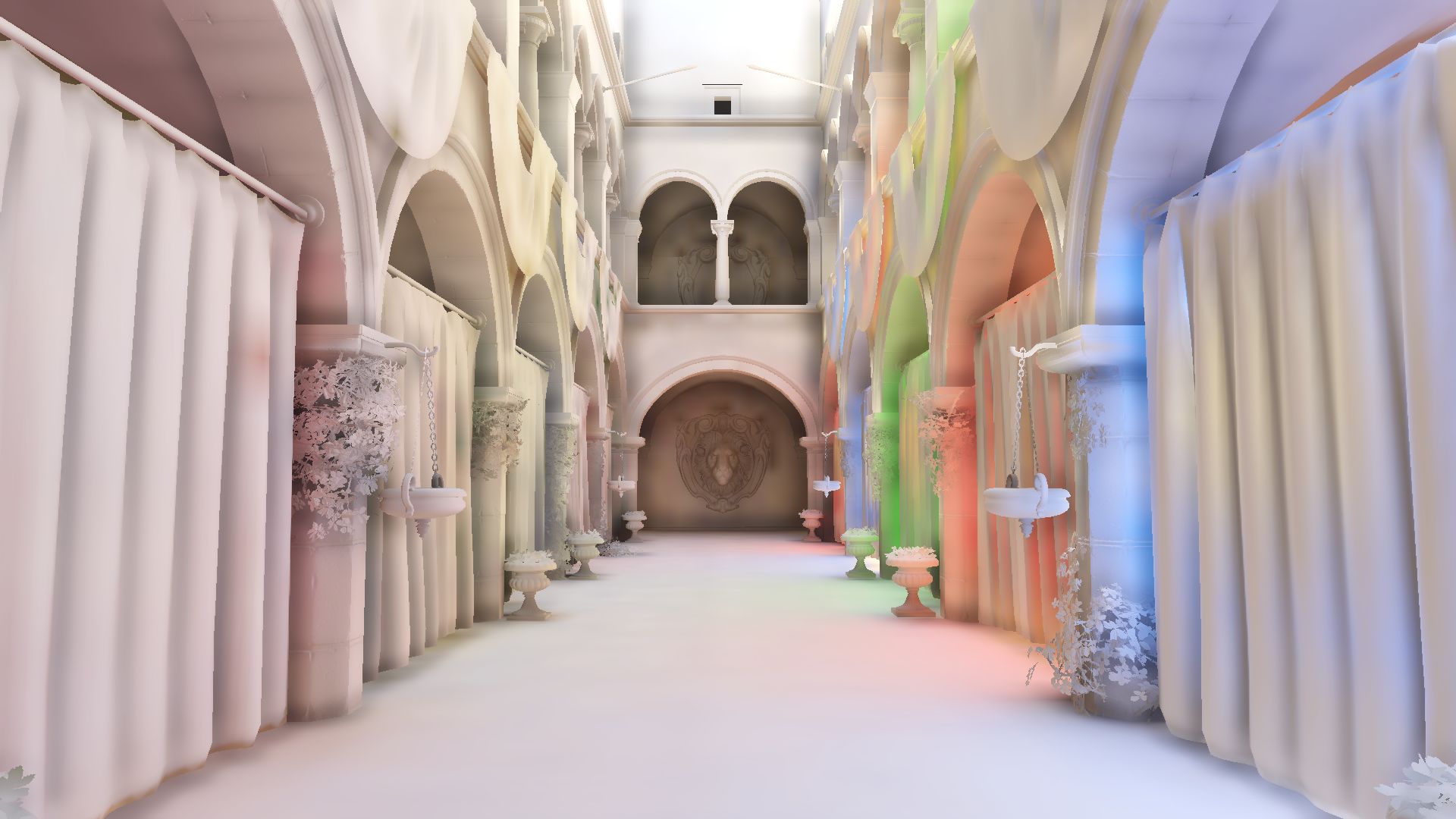 |
Fig. 6. Indirect diffuse lighting and sky light (left). Indirect diffuse lighting and sky light multiplied by SSAO (right).
 |
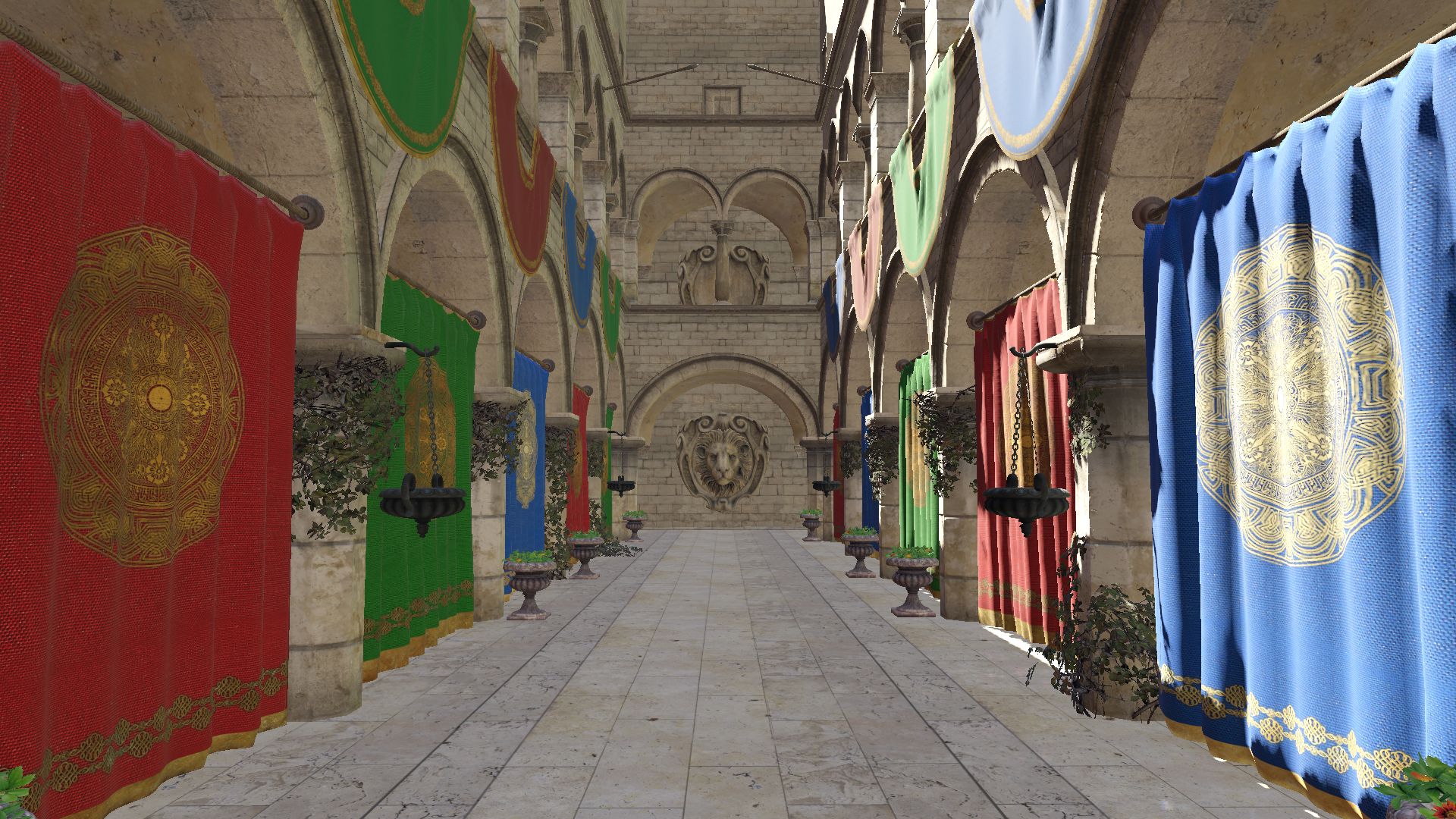 |
Fig. 7. Final shading result with presented GI method (left). Compare to flat lighting with fixed spherical harmonics (right).
4.1 Updating scene voxels representation from g-buffer
The core idea is to stochastically choose some visible screen pixels to update our voxel scene representation. We can potentially discard some pixels based on their g-buffer properties (such as dynamic object pixels, based on dynamic bit or pixel screen motion vectors, to avoid adding dynamic objects to static scene representation). We then light these pixels based on their position, albedo, normal, roughness (or any other set of shading properties stored in g-buffer) and current lighting information, including our irradiance map with indirect lighting (adding multiple bounce information, Figure 8). Most modern deferred lighting techniques such as tiled deferred or clustered deferred allows a re-lighting of all chosen pixels in one dispatch, but even vanilla deferred engines are capable of supporting this re-lighting (but, as in a creating deferred light buffer, we will need to dispatch a call for each light). Our engine relies on clustered deferred lighting, so we have only one dispatch call. Depending on particular engine implementation, it is also possible to just obtain directly light buffer information from the already resolved g-buffer. We made this implementation in the prototyping stage, but in the production implementation we ended up not doing it, since our engine performs all atmospheric scattering in the same pass as resolving a g-buffer. When a chosen pixel is lit, we exponentially average with all current voxels it belongs to (one voxel in each nested 3d-grid) in our voxel scene representation. Exponential averaging weight depends on voxel state (if it is invalid, i.e. never updated, we write without averaging). We ignore potential overwriting of the same voxel multiple times, although it can be solved with atomic operations, but it would also require maintaining an additional ’weight’ array and additional dispatch, and it doesn’t seem worth it (although not hard to implement).
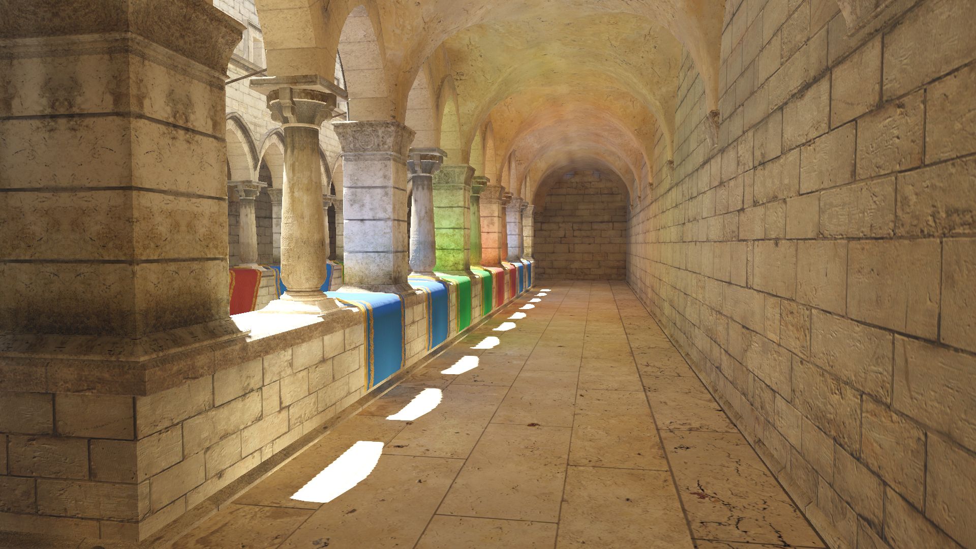 |
Fig. 8. Ceiling is lit only with second and third bounces. Colored third bounce on the floor
The total amount of pixels defines the speed of convergence and the total performance cost of algorithm but this part of the solution is very fast, even a hundred thousand pixels requires less than 0.2 msec on modern hardware GTX 1070, and it scales linearly with the number of pixels. We have chosen this number to be 32768 or smaller.
4.2 Fill-in new scene representation voxels
Although it is not required by algorithm to fill-in such voxels anyhow (except for clearing it’s opacity), setting them to anything reasonable can significantly speed up temporal convergence. If there is no information in newly added scene voxels, raycasting will allow light to travel through them, and this will cause light bleeding (while aesthetically over darkening is preferred over light bleeding). So, there are several ways to address this issue, each of which requires additional information about the scene:
-
Heightmaps around the camera. Most games with large scenes do have heightmap(s) of a level, potentially streamed or generated around the player. Some of them also have some kind of material data for such heightmaps (albedo, roughness). Any of this information is helpful to fill in incoming scene voxels. Heightmaps give us normal and world positions and all voxels that are lower than the lowest heightmap can be filled in with reasonable color and opacity.
-
Shadow data. Any currently available shadow data (such as cascaded shadow maps) can be used to shadow incoming voxels. Some games [Schulz 2014] have shadow data for the whole level.
-
Collision models. Most games do have some simplified collision models representing the world. Since we know on the CPU side of our algorithm the bounding boxes of fresh incoming voxels we need to fill in, we can use any kind of GPU voxelization and fill in these voxels with collision data information. Although collision data typically has no additional information besides pure geometrical data, but normal can be extracted from geometrical data with gradients, and we can assume albedo to be "very dark grey".
-
Of course, if we can use any kind of actual rendering models (including low LOD), we will be able to fill in scene voxels with good and correctly lit (correct materials) data, like [Panteleev 2014].
Although neither of these methods are required for an algorithm to work, any of them will help speed up temporal convergence. The most important part would be to have correct opacity data as it prevents light bleeding. In our engine we use all of the above methods to a certain degree (only few real models, few (biggest) collision models, and heightmap), but the algorithm performs well even with only heightmap and collision. If we do discard some of the scene voxels on a regular basis (see Invalidating/Discarding scene representation voxels), we can also fill-in finer levels with its coarser grid neighbor and speed up the toroidal update of finer levels of the grid.
4.3 Invalidating/Discarding scene representation voxels
It is not required to remove scene voxels for static environments. However, if there are certain changes in scene geometry it may be needed to invalidate a voxels scene representation. In the simplest scenario (like destruction), we can invalidate all voxels in the bounding box of changed geometry (and "fill-in" data). If there are some slow animations we can discard scene voxels on a regular basis, by stochastically checking existing visible (fully in frustum) scene voxels and checking if the whole box is visible against the depth buffer and removing them (set opacity and color to zero).
4.4 Ajure geometry (such as foliage)
| Open fullscreen | Open fullscreen |
If we have opaque geometry which is very sparse in the scene but still mostly transparent (Figure 9), it’s voxel representation becomes inadequate (Figure 10). As voxels are not-transparent to light rays it will cause over darkening of underlying geometry, such as terrain below grass and bushes. There are two ways to mitigate that. First, we can totally skip such pixels in the 5.1 step of the algorithm (based on g-buffer information, such as material information). Second, if we store opacity information in our voxel scene representation (as a separate volume texture or alpha channel of the scene voxel data) we can allow semi-transparent voxels in the scene. In this case, the ray traversal 4.3 algorithm should be modified to well-known accumulate-and-extinct light modification (such as in [Crassin et al. 2011]). In the 5.1 step of the algorithm, if a semitransparent pixel has been found, we can skip it’s voxelization if it’s corresponding scene voxel is already defined as completely opaque, or do not update it’s opacity (but update color).
Fig. 9. The grassy scene with a lot of sparse foliage (left) and it’s correspondent g-buffer translucency channel (right).
 |
 |
Fig. 10. From top to bottom: Voxel scene representation without translucency fix. Darkening caused by inadequate representation. Voxel scene representation with translucency fix. Result picture is much brighter and greener.
5. SHADING WITH PROPOSED DATA FORMATS
5.1 Diffuse term
Shading with irradiance map defined as regular grid is quite simple and well defined [Hooker 2016] [Silvennoinen and Timonen 2015]. We rely on hardware trilinear filtered ambient cube volume textures. There are 3 textures for 6 directions, since positive and negative directions cannot be required simultaneously for each lit pixel with any normal. We have also tried modified trilinear filtering [McGuire et al. 2017] and [Silvennoinen and Timonen 2015], but do not use it for simplicity and performance reasons. For each pixel we have to lit, we sample only one cascade, choosing the most fine irradiance map level. To avoid a discontinuity seam on the border of each cascade with it’s coarser neighbor we blend with next cascade. Since our irradiance map only has indirect lighting and skylight this step only adds indirect diffuse light and diffuse sky light (Figure 6). For direct lighting we rely on a clustered deferred shading [Olsson et al. 2012] (Figure 7)
5.2 Specular term
The quality of the light cube itself is not sufficient to simulate any fine (glossy) reflection, so we can’t use our irradiance map to produce specular reflections (except the roughest). However, our voxel scene representation is sufficient for getting both gloss reflections and also the intersection of reflected eye ray with scene [Panteleev 2014], in order to correct parallax in specular light probes [Sébastien and Zanuttini 2012].
We use both approaches and mix results depending on the roughness of the surface. Irradiance map is still used to correct brightness in specular map (see [Hooker 2016]).
6. MITIGATING LIGHT BLEEDING
The most noticeable issue with irradiance map defined as regular grid is light bleeding [Hooker 2016]. It is possible to utilize a volume shape method from [Hooker 2016], however, unlike them we just filter position on the border of the convex (moving it inside/outside, if it’s trilinear filtering is violating convex border). We can also additionally adjust trilinear filtering based on normal [Silvennoinen and Timonen 2015].
Light leaking example
| Leaking | No leaking with convex offset filtering |
7. RESULTS AND PERFORMANCE
Total memory footprint can vary from 32mb (see Table 2 and 1) to 62mb. For comparison even precomputed and compressed streamed data of same nature [Hooker 2016] requires just almost twice that memory and most of dynamic GI methods are much more costly. The performance cost (Table 3) is also reasonable. While real-time GI is still high-end feature proposed technique make it reasonable for a broad variety of games, especially for large scenes with dynamic environment. Results can be combined with (and enhanced by) typical screen space techniques producing finer details (such as SSAO and SSGI/SSRTGRI). The performance cost can be significantly eliminated by utilizing async compute. The only phase of algorithm that requires g-buffer is scene representation update phase 5.1.
RTX support can significantly increase the quality, eliminating inadequacy of voxel scene representation during ray casting (but keep it for incoming radiance).
Memory footprint:
|
Irradiance map
(3 cascades) |
13.5mb
|
|
Scene representation
|
16.5m
(33mb with improved quality) |
|
Temporal buffers
|
<1mb
|
|
Total
|
~31Mb
|
Performance breakdown:
|
Movement amortized:
0.1-1msec, but each 8-16 frame |
~0.1msec
|
|
Scene feedback
|
~0.02msec
|
|
Irradiance map update
▪ can be async computed
▪ or even disabled
|
1.2msec
|
|
Lighting additional cost
Full HD |
0.3msec
|
|
Total async or 1-bounce:
Sync N-bounce: (measured on Xbox One) |
0.7msec
~1.6msec |
Conclusion:
Overall, this solution provides consistent indirect lighting with multiple light bounces, adjustable quality, supporting low-end PC to ultra-high-end HW support, all without compromising gameplay. Being this is designed as a dynamic system (where as if you blow up a wall, destroy a building, etc) light needs to flood in, you may also build a fortification and it will produce reflex and indirect shadows. Ultimately, this allows us to not only increase the maximum location size to an unlimited level but also the number of light bounces and the number of light sources with no cost to gameplay on the system. These types of light sources are all supported by that engine with the addition of some volumetric lights, no pre-bake with very small additional asset production overhead, and day/time changes as well as destruction and construction support.
With this solution our game receives innovative and complete solution for lighting, which will make our game shine!
You can view the full GDC presentation on Scalable Real-Time Global Illumination by Anton Yudinsev here.
REFERENCES
- Cyril Crassin. 2012. Voxel Cone Tracing and Sparse Voxel Octree for Real-time Global Illumination. In GPU Technology Conference (link)
- [Crassin et al. 2011] Cyril Crassin, Fabrice Neyret, Miguel Sainz, Simon Green, and Elmar Eisemann. 2011. Interactive Indirect Illumination Using Voxel-based Cone Tracing: An Insight. In ACM SIGGRAPH 2011 Talks (SIGGRAPH ’11). ACM, New York, NY, USA, Article 20, 1 pages (link)
- [Hooker 2016] JT Hooker. 2016. Volumetric Global Illumination at Treyarch. In Advances in Real-Time Rendering (SIGGRAPH ’16). ACM (link)
- [McGuire et al. 2017] Morgan McGuire, Mike Mara, Derek Nowrouzezahrai, and David Luebke. 2017. Real-time Global Illumination Using Precomputed Light Field Probes. In Proceedings of the 21st ACM SIGGRAPH Symposium on Interactive 3D Graphics and Games (I3D ’17). ACM, New York, NY, USA, Article 2, 11 pages (link)
- [McTaggart 2004] Gary McTaggart. 2004. Half-Life 2 / Valve Source(tm) Shading. In Game Developers Conference (link)
- ACM Transactions on Graphics, Vol. 36, No. 4, Article 1. Publication date: July 2017.
- [Olsson et al. 2012] Ola Olsson, Markus Billeter, and Ulf Assarsson. 2012. Clustered Deferred and Forward Shading. In HPG ’12: Proceedings of the Conference on High Performance Graphics 2012 (2012-01-01). Paris, France, 87–96 (link)
- [Panteleev 2014] Alexey Panteleev. 2014. Practical Real-time Voxel-based Global Illumination for Current GPUs. In GPU Technology Conference (link)
- Marco Salvi. 2008. Rendering filtered shadows with exponential shadow maps. Charles River Media, Chapter 4.3, 257–274.
- [Sébastien and Zanuttini 2012] Lagarde Sébastien and Antoine Zanuttini. 2012. Local Image-based Lighting with Parallax-corrected Cubemaps. In ACM SIGGRAPH 2012 Talks (SIGGRAPH ’12). ACM, New York, NY, USA, Article 36, 1 pages (link)
- [Silvennoinen and Timonen 2015] Ari Silvennoinen and Ville Timonen. 2015. Multi-Scale Global Illumination in Quantum Break. In Advances in Real-Time Rendering (SIGGRAPH ’15). ACM (link)
- Bart Wronsky. 2014. Assassin’s Creed 4: Black Flag Digital Dragons. In Game Developers Conference (link)